its weight. This measure plays a significant in indicating the relationship between the two vertices it connects. For example the graph in figure 1 has 4 vertices connected by 4 edges each of which have a weight associated with it.
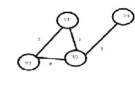
Figure 1.0
International Journal of Scientific & Engineering Research, Volume 5, Issue 5, May-2014 1230
ISSN 2229-5518
Graph-based Data Mining: A New Approach for
Data Analysis
Nandita Bothra, Anmol Rai Gupta
—————————— ——————————
Graph theory is the subject that deals with graphs. Graph theory has found its applications in many areas of Computer science. Data mining is one of those fields where concepts of graph theory have been applied to a large extent. Data mining (Han et al, 2006) is the subject which deals in extraction of knowledge from the available data. Various algorithms are applied which help in the analysis and establishment of relationship between the entities. Apart from finding relationship between various entities of data, data mining algorithms have been widely used to perform cluster analysis as well. Mining large datasets with conventional algorithms is tough because of polynomial time complexities. Graph mining and management has become an important topic of research recently because of numerous applications to a wide variety of data mining problems in computational biology, chemical data analysis, drug discovery and communication networking.
Traditional data mining and management algorithms such
as clustering, classification, frequent pattern mining and indexing have now been extended to the graph scenario. Graph data mining has shown better results in terms of time complexities and thus is a preferred technique when handling large data sets.
Definition 1 (Graph): A graph can be defined in an abstract way using vertices or nodes, edges connecting the nodes and mapping of the edges from one vertex to the other. A weighted graph (West, Douglas B, 2005) is one in which a
number is associated with each edge which is often called
its weight. This measure plays a significant in indicating the relationship between the two vertices it connects. For example the graph in figure 1 has 4 vertices connected by 4 edges each of which have a weight associated with it.
Figure 1.0
Definition 2 (Subgraph): A graph G’: {V’, E’} is said to be a subgraph of G: {V, E} if and only if it satisfies the following two conditions.
i) V’ ϵ V
ii) E’ ϵ E
Definition 3: (Graph Transaction) A graph G is referred to as a graph transaction or simply a transaction, and a set of
graph transactions GD, where GD = {G1 , G2 … Gn}, is
referred to as a graph database.
Definition 4: (Support) Given a graph database GD and a graph Gs , then support of Gs is defined as
IJSER © 2014 http://www.ijser.org
International Journal of Scientific & Engineering Research, Volume 5, Issue 5, May-2014 1231
ISSN 2229-5518
𝑁𝑜.𝑜𝑓 𝑡𝑟𝑎𝑛𝑠𝑎𝑐𝑡𝑖𝑜𝑛𝑠 𝑖𝑛𝑣𝑜𝑙𝑣𝑖𝑛𝑔 𝐺𝑠
Sup (Gs ):
𝑇𝑜𝑡𝑎𝑙 𝑛𝑜.𝑜𝑓 𝑡𝑟𝑎𝑛𝑠𝑎𝑐𝑡𝑖𝑜𝑛𝑠 𝑖𝑛 𝐺𝐷
![]()
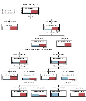
data in a better way, we converted it into a tree format.
In this paper, we have implemented the Apriori Algorithm (written below) on the procured dataset and have established various association rules which affect the men’s fertility.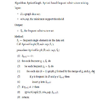
After applying Apriori algorithm and determining the association rules, web graphs were constructed for the data which depicts the data in weighted graph format. The research has been further extended to neural network analysis which aims at considering affect of those attributes which have values over range instead of binary values. We have also performed K means clustering which depicts the
density of records in different areas. To understand the
Figure 2.0
4.1 Description of dataset
We procured the dataset from UCI Machine learning repository which contains information about semen samples given by 100 volunteers and was analyzed according to the WHO 2010 criteria. Sperm concentrations are related to socio-demographic data, environmental factors, health status, and life habits. The data was donated to UCI repository on Jan 17, 2013.
Attribute information is tabulated below
Attribute | Value |
Season in which the analysis was performed | Winter, Spring, Summer, Fall (-1,-0.33,0.33,1) |
Age at the time of analysis. | 18-36 (0, 1) |
Childish diseases (i.e. , chicken pox, measles, mumps, polio) | 1) Yes, 2) no. (0, 1) |
Accident or serious trauma | 1) Yes, 2) no. (0, 1) |
Surgical intervention | 1) Yes, 2) no. (0, 1) |
High fevers in the last year | 1) Less than three months ago, 2) more than three months ago, 3) no. (-1, 0, 1) |
IJSER © 2014 http://www.ijser.org
International Journal of Scientific & Engineering Research, Volume 5, Issue 5, May-2014 1232
ISSN 2229-5518
• High fevers: Fever affects the production and quality of the sperm count. This usually takes weeks to recover from.
• Alcohol consumption: Alcohol is considered toxic to
the sperm and overuse can cause infertility.
• Smoking habit: Smoking results in approximately
700 chemicals entering the body. These damage the
sperms and make them less likely to fertile the egg.
• Number of hours spent sitting per day: Sitting for long
hours heats up the testicles and lack of exercise adds on to it, making the man infertile.
Following are the various risk factors that have been
considered in the given dataset which are believed to affect the men’s fertility.
• Childish diseases: When infected with a disease like chicken pox, measles, mumps or polio the infection might spread to other parts of the body. This may affect the testicles and result in testicular shrinkage and infertility.
• Accident or serious trauma: Injury to the testicles
during an accident can cause fertility. Serious trauma or depression also results in decrease in sperm count and hence causes infertility.
• Surgical intervention: Some males go through
surgical intervention to improve their fertility.
Figure 3.0
Apriori algorithm has been used for classification for datasets and establishment the association rules in between the attributes on the basis of two measures: minimum support and minimum confidence. For generating item sets we have used the existing Apriori algorithm and further we have extended the concept to Apriori graph mining technique.
The following item sets in Table 1.4 were generated by taking minimum support= 20%.
After procuring whole of the data we converted it into table format. Figure 3.0 shows information for 15 samples.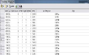
Attribute | Count of yes | Total instances | Support % |
Accident | 44 | 100 | 44 |
Childish diseases | 87 | 100 | 87 |
Surgery | 51 | 100 | 51 |
Since all the three attributes fulfill the minimum support criteria, we calculated the 2 item set by taking 2 attributes at a time.
IJSER © 2014 http://www.ijser.org
International Journal of Scientific & Engineering Research, Volume 5, Issue 5, May-2014 1233
ISSN 2229-5518
To generate association rules we took minimum confidence as 90%. Following rules were generated.
Further we go for computation of 3 frequent item set.
Interpretation of Table1.7 is if e.g. for the last association
rule where antecedent is accident and childish disease and the consequent is Output, it means 92.683% of the people have undergone surgery and have had childish diseases are fertile.
The graph in figure 4.0 was constructed using all the flag attributes. Every flag attribute was given allotted two nodes; one representing either yes or 1 and the other representing either no or 0.
Figure 4.0
The edges in the graph can be classified into three categories: Heavy link, medium link and weak link. This
classification was made on the basis of the count
(weight) of that particular edge. It has been
summarized below.
The purpose of going one step ahead of weighted graph was to create visual effect of the count and making it easier for analysis. As one can see from the graph itself, the strongest link is the edge between Output=Yes and Childish Diseases=1.
IJSER © 2014 http://www.ijser.org
International Journal of Scientific & Engineering Research, Volume 5, Issue 5, May-2014 1234
ISSN 2229-5518
On constructing the neural network for our data set, we got the relative importance of the parameters that we used on the output (i.e., the decision whether a man has normal fertility or not. The neural net uses minimal statistical or mathematical knowledge and shows the output by the way the human mind processes the information. After running our data sets in the Neural Net it was found that Alcohol has the most importance in determining the fertility, followed
by smoking and the season in which the test was taken.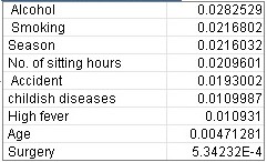
Table 1.3: Neural Net Results
Table 1.2
The importance of neural network in this research is that it represents the effect of those attributes which have a range of values.
Clustering in graphs is well researched topic and many algorithms have been proposed by various authors. In graph related clustering, there are two possible approaches:
1. Determination of dense node clusters in a single large
graph. 2. There are multiple graphs of modest size and one wants to cluster those graphs as objects. In this research,
we followed the first approach in which we implemented K means clustering algorithm. The reason for choosing K means clustering was that it is an effective partitioning clustering algorithm. As explained by Macqueen4, The procedure follows a simple and easy way to classify a given data set through a certain number of clusters fixed a priori. Every cluster is defined with a centroid and each object is assigned to the group which has the closest centroid.
While implementation, we specified number of clusters to be extracted as 5.
IJSER © 2014 http://www.ijser.org
International Journal of Scientific & Engineering Research, Volume 5, Issue 5, May-2014 1235
ISSN 2229-5518
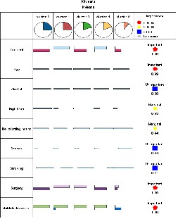
Figure 5.0
Approaches to Graph mining have been categorized into 5 categories (Takashi et al): Greedy based approach, mathematical graph theory based approach, Inductive logic programming, Inductive database based approach and kernel function based approach.
As Takashi et al have explained “Apriori Graph mining falls under mathematical graph theory based approach because this approach mines the large datasets based on support measures. One vertex is assigned to each of the graphs from the frequent graphs and then frequent graphs which are relatively larger in size are searched in bottom up approach. Let the number of vertices contained in a graph
be its “size", an adjacency matrix of a graph whose size is k be Xk, the ij-element of Xk, xij and its graph, G (Xk). AGM can handle the graphs consisting of labeled vertices and labeled edges. The vertex labels are defined as Np (p=1…α) and the edge labels, Lq(q = 1…β). Labels of vertices and edges are indexed by natural numbers for computational efficiency. The AGM system can mine various types of sub graphs including general subgraph, induced subgraph, and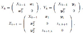
connected subgraph, ordered sub tree, unordered subtree and subpath. The candidate generation of frequent induced subgraph is done as follows. Two frequent graphs are joined only when the following conditions are satisfied to generate a candidate of frequent graph of size k+1. Let Xk and Yk be adjacency matrices of two frequent graphs G(Xk ) and G(Yk) of size k. If both G (Xk) and G (Yk) have equal elements of the matrices except for the elements of the kth row and the kth column, then they are joined to generate Zk+1 as follows.
Where Xk-1 is the adjacency matrix representing the graph whose size is k-1, xi and yi(i = 1, 2) are (k-1)*1 column vectors. The elements z k,k+1 and zk+1,k represent an edge label between kth vertices of Xk and Yk . Their values are mutually identical because of the diagonal symmetry of the undirected graph. Here, the elements z k,k+1 and zk+1,k of the adjacency matrix Zk+1 are not determined by Xk and Yk . In case of an undirected graph, two possible cases are considered in which 1) there is an edge labeled Lq between the kth vertex and the k+ 1th vertex of G(Zk+1 ) and 2) there
is no edge among them. Accordingly β+1 adjacency
matrices whose (k, k+1) element and (k + 1, k)-element are “0" and “Lq" are generated. Xk and Yk are called the first matrix and the second matrix to generate Zk+1 respectively. Because the labels of the kth nodes of Xk and Yk are the same, switching Xk and Yk, i.e., taking Yk as the first matrix and Xk as the second matrix, produces redundant adjacency matrices. In order to avoid this redundancy, the two adjacency matrices are joined only when the following condition is satisfied.
code(the first matrix) ≤ code(the second matrix)
The adjacency matrix generated under these constraints is a "normal form". The graph G of size k+1 is a candidate frequent graph only when adjacency matrices of all induced subgraphs whose size are k are confirmed to be frequent graphs. If any of the induced subgraphs of G(Zk+1 ) is not frequent, Zk+1 is not a candidate frequent graph, because
any induced subgraph of a frequent graph must be a
frequent graph due to the anti-monotonicity of the support.
This check to use only the former result of the frequent graph mining is done without accessing the graph data set. After the generation of candidate subgraphs, their support is counted by accessing the data set. To save computation for the counting, the graphs in the data set are represented in normal form matrices, and each subgraph matching is
IJSER © 2014 http://www.ijser.org
International Journal of Scientific & Engineering Research, Volume 5, Issue 5, May-2014 1236
ISSN 2229-5518
made between their normal forms. This technique significantly increases the matching efficiency. The process continues in level-wise manner until no new frequent induced subgraph is discovered.”
In this research, we analyzed various factors that affect the men’s fertility. Various association rules were established which can help can help the doctors identify multiple cause to infertility. As the concept of basket analysis was further extended to Apriori Graph Mining, it makes the data mining of large datasets highly effective by making use of adjacency matrixes as explained. This research can be very helpful in the field of ontology and medical sciences. It can be extended to study of various cancers, liver problems
with risk factors as alcohol and fats. It can also be extended
to the study of genetic diseases and determining the probability of occurrence of those diseases in the child. Also, we plan to implement it on the datasets containing information of various districts with their population and diseases which can help the Ministry of Health to determine the prevalent diseases in particular areas and take appropriate steps.
7 REFERENCES
[1] J. Cook and L. Holder. Substructure discovery using minimum description length and background knowledge. J.Artificial Intel. Research, 1:231-255, 1994.
[2] M. Kuramochi and G. Karypis. Frequent subgraph discovery. In ICDM'01: 1st IEEE Conf. Data Mining, pages
313-320, 2001.
[3] H. Mannila and H. Toivonen. Discovering generalized episodes using minimal occurrences. In 2nd Intl. Conf. Knowledge Discovery and Data Mining, pages 146-
151,1996.
[4] C. Aggarwal, P. Yu. Online Analysis of Community
Evolution in Data Streams. SIAM Conference on Data Mining,
2005
[5] D. Cook, L. Holder. Mining Graph Data, John Wiley & Sons Inc, 2007.
[6] MacQueen, J. B. (1967). "Some Methods for classification and Analysis of Multivariate Observations". 1. Proceedings
of 5th Berkeley Symposium on Mathematical Statistics and
Probability. University of California Press. pp. 281–
297. MR 0214227. Zbl 0214.46201. Retrieved 2009-04-07. [7] West, Douglas B. (2001). Introduction to Graph
Theory (2ed). Upper Saddle River: Prentice Hall. ISBN 0-13-
014400-2.
[8] P. Cheeseman and J. Stutz, “Bayesian Classification (AutoClass): Theory and Results,”Advances in Knowledge Discovery and Data Mining, U.M. Fayyad et al., eds., MIT Press,Cambridge, Mass., 1996, pp. 153–180.
[9] L. Dehaspe and H. Toivonen. Discovery of frequent datalog patterns. Data Mining and Knowledge Discovery,
3(1):7(36), 1999.
[10] Jiawei Han and Micheline Kamber, Data Mining Concepts and Techniques, Second Edition, Morgan Kauffman Publishers, 2009.
[11] M. Zaki. Efficiently mining frequent trees in a forest. In
8th Intl. Conf. Knowledge Discovery and Data Mining, pages 71(80), 2002.
[12] D. J. Cook and L. B. Holder: Graph-Based Data Mining, IEEE Intelligent Systems, 15(2), 32-41, 2000.
[13] A. Inokuchi, T. Washio and H. Motoda, An Apriori-
based Algorithm for Mining Frequent Substructures from Graph Data, Proceedings of the European Conference on Principles and Practice of Knowledge Discovery in Databases, 2000.
[14] X. Yan and J. Han, gSpan: Graph-Based Substructure
Pattern Mining, Proceedings of the IEEE International
Conference on Data Mining (IEEE ICDM), 2002.
[15] T. Washio and H. Motoda, “State of the art of graph based data mining,” SIGKDD Explor. Newsl., vol. 5, no. 1, pp. 59–68, 2003.
This entire research has been based on the dataset procured from UCI Machine library repository. We are highly indebted to the organization without which this research wouldn’t have been possible. We are also grateful to developers of SPSS Clementine 11.1. We will also like to thank Prof Geetha Mary A and Dr. Selvakumar R for their incredible help throughout this research.
IJSER © 2014 http://www.ijser.org